A Lightweight Complex CNN + SE for Co-Freq. SC-BSS

01

Key Findings

Four things you should take away from this paper.

First phase-preserving, real-gated complex SE

To our knowledge, the first SE-style channel-attention mechanism designed natively for complex-valued feature maps. Real-valued gating weight preserves the I/Q phase coupling critical for demodulation.

235K params, 5-seed evaluation

3.5× smaller than the comparable Complex Conv-TasNet, 28× smaller than CNSE. Five seeds per configuration with paired Wilcoxon tests; no comparison reaches $\alpha = 0.05$.

Output-collapse is a per-seed hazard

Without C-SE, 4 of 5 seeds collapse to a degenerate solution ($\text{SIR}\approx20 dB$). With C-SE, only 2 of 5 collapse. The failure is structural, not parameter-driven.

Generalises to the co-frequency limit

Trained on $\Delta f \sim U(0, 5)$ Hz, the model hits $\text{SDR}=3.33 dB$ at the unseen $\Delta f=0$ Hz limit and holds $\text{SDR}\approx3.3 dB$ across the entire $[0, 500]$ Hz range.

02

Background & Concepts

Everything you need to read the rest of the page. Skim if you are already familiar with SC-BSS, complex-valued networks, and PIT losses.

2.1

What is single-channel blind source separation?

A radio receiver records one signal that is the sum of two or more unknown sources. Given the single mixed signal, recover the originals. With only one sensor, classical methods like ICA have more unknowns than equations—they cannot work in the single-channel case at all.

Deep learning sidesteps the underdeterminism by learning a prior over what the sources look like—for communication signals, that prior is "a sequence of constellation symbols shaped by a pulse filter and carried by a slow oscillator." Once the prior is baked into the network, separation becomes a Bayesian inference problem.

Where this matters. Spectrum surveillance, cognitive radio, electronic-warfare receivers, and non-orthogonal multiple access (NOMA) in 5G/6G.

2.2

What is the "co-frequency" regime?

Two transmitters on the same nominal frequency produce two I/Q waveforms whose carrier frequencies differ by only a few hertz—much less than the symbol rate. Classical time-frequency masking fails here because the two spectra overlap completely. The only handle left is the fine I/Q structure inside the shared spectrum.

In this paper the carrier separation is exactly $|\Delta f_1 - \Delta f_2| = 5 Hz$ at training time. The signal bandwidth is roughly $\sim 1 kHz$, so the two carriers overlap by more than 99.5%. We also test the extreme co-frequency limit $\Delta f = 0 Hz$ after retraining on $U(0, 5)$ Hz.

2.3

Why "complex-valued" networks?

A digital communication signal is a complex baseband waveform: $s(t) = I(t) + j Q(t)$. Treating $(I, Q)$ as two independent real channels discards the algebraic structure: the phase $\varphi = \mathrm{atan2}(Q, I)$ encodes the constellation symbol, and the magnitude encodes the pulse envelope.

A complex-valued layer respects this structure. Complex convolution, complex batch-norm, and complex ReLU all follow the standard real/imaginary decomposition but keep the two parts coupled—the network can rotate or reflect the constellation without learning two redundant coordinate transformations.

Constellation view. Plotting every $(I, Q)$ sample at the symbol-rate produces the constellation diagram—a 4-point cloud for QPSK, a 16-point cloud for 16QAM. Recovering this structure is what makes the result useful for demodulation.

The three numbers on every chart: SDR, SIR, and SI-SDR

Each measures a different kind of separation error. SDR and SIR anti-correlate: improving one by suppressing interference usually degrades another by distorting the waveform.

$\text{SDR} = 10 \log_{10} \dfrac{\|\alpha \mathbf{s}\|^2}{\|\hat{\mathbf{s}} - \alpha \mathbf{s}\|^2}$: Source-to-Distortion Ratio. Measures total error against the true source—any deviation counts. Use when you care about waveform fidelity (e.g. analog signal reconstruction).
$\text{SIR} = 10 \log_{10} \dfrac{\|\alpha \mathbf{s}\|^2}{\|\hat{\mathbf{s}}_{\perp}\|^2}$: Source-to-Interference Ratio. Measures only the part of the estimate that is orthogonal to the source—residual interference from the other source. Ignores self-distortion. Use when you care only about cross-talk.
$\text{SI-SDR} = 10 \log_{10} \dfrac{\|\alpha \mathbf{s}\|^2}{\|\hat{\mathbf{s}} - \alpha \mathbf{s}\|^2}$ with $\alpha = \mathbf{s}^{\top}\hat{\mathbf{s}} / \|\mathbf{s}\|^2$: Scale-Invariant SDR. Removes the arbitrary global gain before measuring. Equivalent to projecting onto the source direction. The dominant term in our training loss.

Why we report all three. SDR alone hides whether the residual error comes from cross-talk or waveform distortion. The combined MSE + negative-SI-SDR loss is approximately flat in the subspace that trades waveform fidelity for interference suppression, allowing either operating point to be reached depending on early-training randomness. In Paper 2 (the companion CDP-Mamba paper) this manifests as a two-attractor landscape; here, the same effect shows up as the output-collapse regime—a seed that converges to a high-SIR / low-SDR degenerate solution.

The output-collapse failure mode

In our 5-seed evaluation, two of the baselines (no-SE complex CNN, real-valued CNN) and one seed each of the proposed C-SE and Conv-TasNet converge to a degenerate solution: the decoder learns to produce near-zero masks, achieving low MSE by suppressing all output. The signature is unambiguous:

Working regime. $\text{SDR} \approx 2.5 dB$, $\text{SIR} \approx 6 dB$. The model distributes error evenly between distortion and residual interference. SER is around 0.53. This is what the proposed C-SE achieves on 3 of 5 seeds.
Collapse regime. $\text{SDR} \approx 1.6 dB$, $\text{SIR} \approx 20 dB$. The model learned to aggressively zero out interference, at the cost of distorting its own output. The waveform is no longer faithful. 2 of 5 C-SE seeds, 4 of 5 no-SE seeds, 2 of 5 real-valued seeds, and 1 of 3 Conv-TasNet seeds land here.

Both regimes sit at comparable loss values—one is not "better" than the other. The training trajectory (controlled by initial weights, dropout, data-order randomness, and GPU non-determinism) selects one apparently at random. Without multi-seed evaluation, you cannot tell which regime a single number came from.

Why this is a Paper 1 problem too. The collapse rate is structural to the complex-CNN training without attention: a model that can suppress all output cheaply will sometimes do so. The C-SE block provides per-channel gain factors that prevent any channel from being permanently muted, reducing the collapse rate from 4/5 to 2/5. It is not a complete fix; a more robust solution would require a different loss or architectural change.

03

Method

Complex features end-to-end. A real-valued channel weight gates the complex feature map while preserving phase.

ComplexLightweightSepNet system overview

Figure 1. System overview. The complex mixture is encoded by a strided complex convolution, projected through a C-SE attention bottleneck, processed by $N$ complex residual blocks with C-SE attention, and decoded through a complex mask head. Total parameters: 235K.

Complex Squeeze-and-Excitation (C-SE)

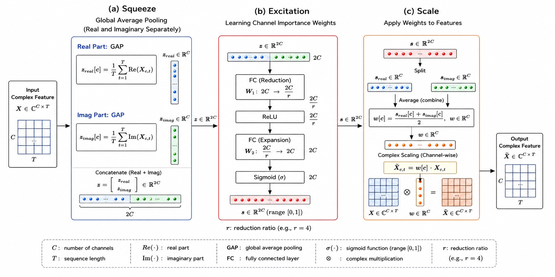
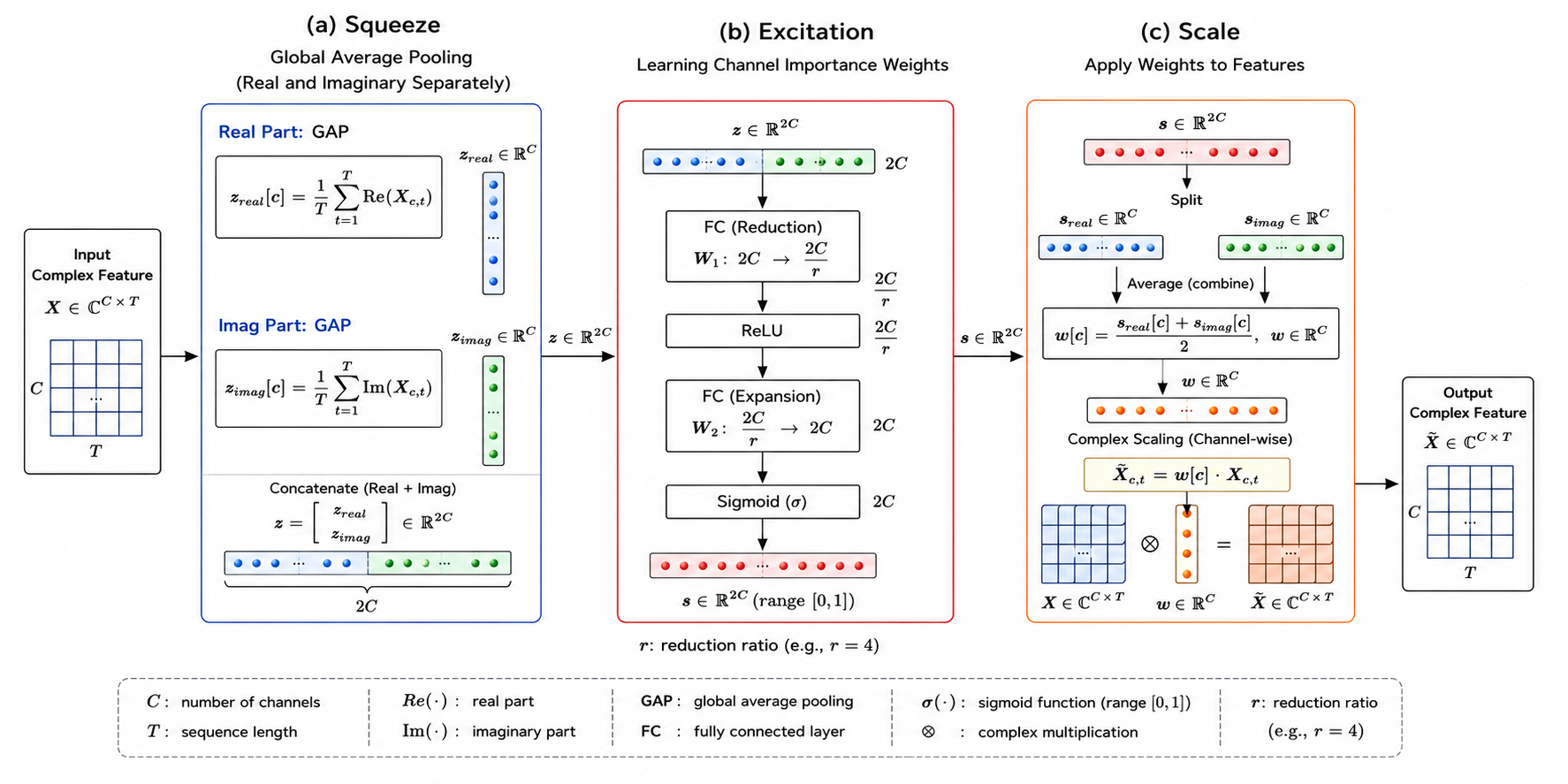
The naive lift of SE to complex data treats I and Q as two independent real channels and discards the multiplicative coupling that encodes constellation structure. Our C-SE design has three steps:

Squeeze. Global-average-pool the real part and the imaginary part separately to produce two channel-wise descriptors $\mathbf{z}_r, \mathbf{z}_i \in \mathbb{R}^{C}$. Concatenate to a single vector $\mathbf{z} = [\mathbf{z}_r, \mathbf{z}_i] \in \mathbb{R}^{2C}$.
Excite. Pass $\mathbf{z}$ through a 2-layer MLP (FC → ReLU → FC → Sigmoid) to produce a 2C-dim vector; split it into $\mathbf{s}_r, \mathbf{s}_i \in [0, 1]^{C}$.
Scale. Apply a real-valued weight to the complex feature: $\tilde{\mathbf{x}}_c = \frac{\mathbf{s}_r + \mathbf{s}_i}{2} \cdot \mathbf{x}_c$. The average of the two sigmoids is used because applying separate real and imaginary weights would rotate the constellation. Averaging preserves phase while adjusting magnitude.

Why not a complex-valued weight? A complex sigmoid gate $\sigma(\mathbf{w}_r) + j\sigma(\mathbf{w}_i)$ would rotate the constellation depending on its phase. The averaged-real design avoids that rotation by construction—phase is preserved by design. The ablation in Table 4 confirms that the choice of scaling mode does not matter for accuracy: real, complex-mean, and separate-real-imaginary all reach $\text{SDR} \approx 2.75 dB$ within $0.01 dB$ spread.

①

Strided complex encoder $(k{=}16, \text{stride}\,8)$

A single strided complex convolution compresses the $T{=}4096$-sample complex waveform into a $512$-step feature sequence (8× temporal compression). The 8× downsample is matched to the symbol rate—we keep about one feature vector per symbol.

②

Complex residual blocks $\times 4$ with C-SE attention

Four complex residual blocks (Conv → BN → ReLU → Conv → BN → C-SE → ReLU + residual). Each block contains a C-SE attention step. The blocks together carry the bulk of the 235K parameters.

③

Complex mask decoder $(1 \times 1$ conv → sigmoid-bounded magnitude$)$

The decoder is a 1×1 complex convolution producing two complex masks $\mathbf{m}_1, \mathbf{m}_2$. The estimates are $\hat{\mathbf{s}}_k = \mathcal{D}(\mathbf{m}_k \odot \mathbf{E})$ where $\mathcal{D}$ is the transposed-encoder mirror. The mask-bounded magnitude keeps the output in a stable range during training.

04

Main Results

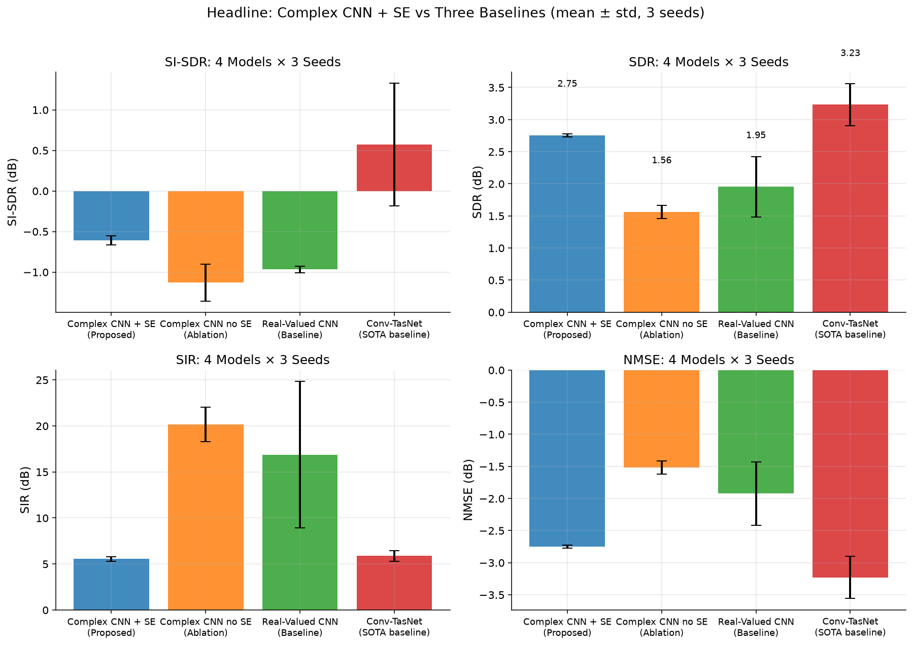
Five random seeds (42–46) for the proposed C-SE and the matched baselines; three seeds for the cross-domain baselines. SNR = 10 dB, all modulation pairs averaged.

Headline comparison (4 metrics, 5 seeds)

Source: paper Figure 1

C-SE matches the parameter-matched real-valued baseline on SI-SDR and SDR, while consuming 3.5× fewer parameters than Conv-TasNet. The wide error bars on SIR (especially for the no-SE and Real-Valued baselines) reflect the output-collapse regime some seeds converge to.

Table 1 · Per-modulation-pair detail (3 seeds at SNR = 10 dB)

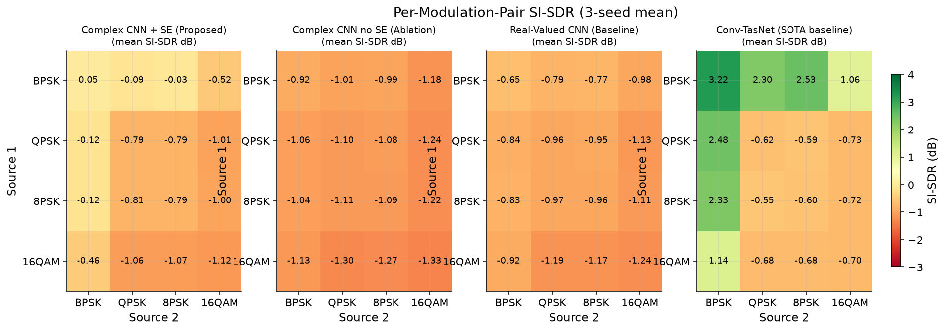
Model	BPSK–BPSK (easiest)		16QAM–16QAM (hardest)
	SDR (dB)	SER	SDR (dB)	SER
Complex CNN + SE (Proposed)	3.00	0.260	2.52	0.837
Complex CNN (no SE)	1.59	—	1.49	—
Real-Valued CNN	2.02	—	1.86	—
Complex Conv-TasNet	4.25	0.230	2.69	0.833

On the easiest case (BPSK–BPSK), Conv-TasNet excels with $\text{SDR}=4.25 dB$. On the hardest case (16QAM–16QAM), the proposed C-SE matches Conv-TasNet ($2.52 dB$ vs. $2.69 dB$, difference only $0.17 dB$) and the SER is nearly identical ($0.837$ vs. $0.833$).

Table 2 · 5-seed evaluation with Wilcoxon tests (all pairs, SNR = 10 dB)

Model	Params	N	SI-SDR (dB)	SDR (dB)	SIR (dB)	Paired ΔSDR	Paired p
Complex CNN + SE (Proposed)	235K	5	−0.66 ± 0.09	2.31 ± 0.62	11.35 ± 7.96	—	—
Complex CNN no-SE (matched, H=70)	242K	5	−0.98 ± 0.06	1.81 ± 0.48	18.01 ± 6.79	+0.50	0.125
Real-Valued CNN (matched, H=80, L=12)	237K	5	−0.94 ± 0.07	2.20 ± 0.59	11.60 ± 8.24	+0.11	0.0625
Complex Conv-TasNet	817K	3	0.58 ± 0.92	3.23 ± 0.40	5.88 ± 0.70	−0.48	0.25
CNSE (scaled, Hou & Gao 2022)	6.69M	3	1.99 ± 0.21	2.38 ± 0.91	16.65 ± 8.65	+0.38	0.5
S4-UNET (scaled, Gao et al. 2026)	1.57M	3	0.01 ± 0.12	3.05 ± 0.00	5.77 ± 0.17	−0.30	0.25

Honest conclusion: no comparison against C-SE reaches statistical significance at $\alpha = 0.05$. The smallest $p$-value is $0.0625$ (against the matched real-valued baseline), which is the smallest attainable two-sided $p$ at $N=5$ pairs. We position C-SE as a competitive operating point at the $235 K$-parameter scale on the dimensions of partial collapse-resistance, per-parameter efficiency, and predictable runtime—not as a statistically dominant architecture.

Per-modulation-pair SDR heatmap (proposed C-SE)

Source: paper Figure 2

SDR ranges from $2.52 dB$ (16QAM–16QAM, hardest) to $3.00 dB$ (BPSK–BPSK, easiest). The model does not collapse on any particular constellation combination. Difficulty grows with modulation order.

05

Robustness

Trained on $\Delta f = 5 Hz$ and $T=4096$ only. We test how far the same checkpoint extrapolates.

Frequency-offset robustness (5–500 Hz)

Models trained at $\Delta f = 5 Hz$ · evaluated on wider gaps

All models show graceful improvement as the separation increases (sources become more distinguishable in frequency). C-SE maintains a consistent $0.2$–$0.5$ dB gap to Conv-TasNet, narrowing at larger offsets.

Micro-frequency generalisation: trained on $U(0, 5)$ Hz

The unseen co-frequency limit $\Delta f = 0 Hz$ is reached without loss of accuracy

C-SE holds $\text{SDR} \approx 3.3 dB$ across the entire $[0, 500]$ Hz range, including the unseen co-frequency limit $\Delta f = 0 Hz$ ($\text{SDR}=3.33 dB$). The no-SE baseline still collapses to $\text{SIR}\approx21 dB$ at every gap—confirming the gap is structural, not a training-set coverage issue.

Length generalisation (T = 2048, 4096, 8192)

Same checkpoint, no retraining

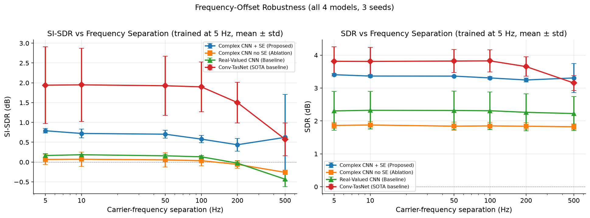
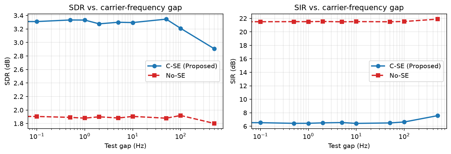
Signal length T	SDR (dB)	SI-SDR (dB)	SIR (dB)	NMSE (dB)
2048 (half)	2.52	−1.31	5.99	−2.52
4096 (train)	3.33	0.58	5.67	−3.33
8192 (double)	2.85	−0.49	6.21	−2.85

The model transfers gracefully across a $4\times$ length range. The $T{=}2048$ drop is expected (fewer symbols per signal window); the $T{=}8192$ drop of $0.48 dB$ is a known limitation of fixed-kernel CNNs (compare with the recurrent SSM in Paper 2, which holds $\text{SDR} \approx 3.1 dB$ at $4\times$ the training length).

06

Ablation Studies

Three questions: does the C-SE block matter? Does the real-vs-complex scale mode matter? Does the pooling strategy matter?

Ablation: C-SE on vs. off (parameter-matched, 5 seeds)

Source: paper Figure 7

C-SE contributes a $0.50 dB$ SDR improvement in the parameter-matched configuration (235K vs. 242K) and reduces the output-collapse rate from 4 of 5 to 2 of 5 seeds.

Ablation: SE scale mode (3 modes, 2-3 seeds each)

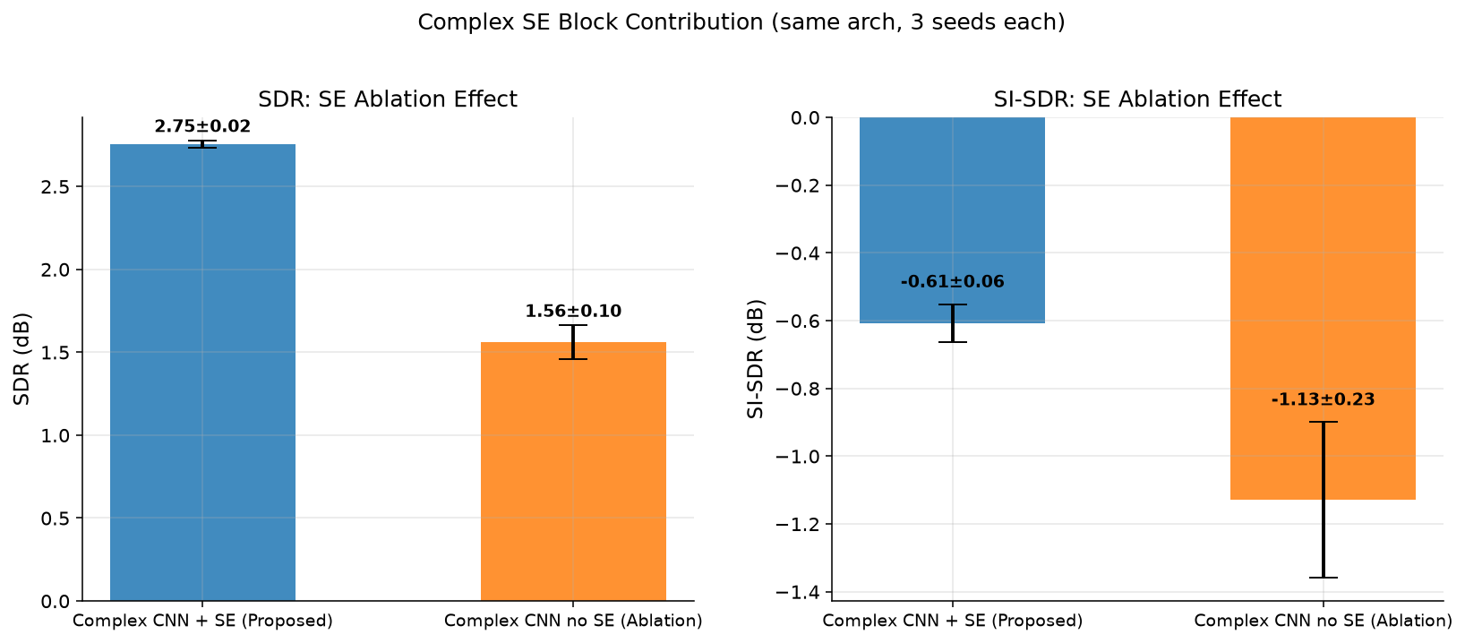
Scale mode	s42 SDR	s43 SDR	SDR (dB)	SER	Description
real (proposed)	2.79	2.74	2.75	0.544	Real weight, average of $\mathbf{s}_r$ and $\mathbf{s}_i$
complex_mean	2.76	2.76	2.76	0.544	Complex-valued weight $\mathbf{s}_r + j\mathbf{s}_i$
separate	2.75	2.77	2.76	0.545	Two independent real weights applied to I and Q separately

All three modes perform nearly identically (SDR spread $\le 0.01 dB$). The simpler real mode is sufficient: the choice between these is not performance-critical. This experiment does not establish that complex phase is irrelevant to SC-BSS in general; the complex_mean variant does not constitute a fair test of complex phase.

Ablation: C-SE squeeze pooling (single-seed, s43)

Pooling	SDR (dB)	SI-SDR (dB)	SIR (dB)	NMSE (dB)	Description
mean (proposed)	2.74	−0.65	5.73	−2.74	$\mu(\text{Re}), \mu(\text{Im})$
power	2.71	−0.66	5.55	−2.71	$\mathbb{E}[\text{Re}^2], \mathbb{E}[\text{Im}^2]$
magnitude	2.74	−0.65	5.74	−2.74	$\mathbb{E}[\|\text{Re}\|], \mathbb{E}[\|\text{Im}\|]$
mean+power	1.58	−0.78	21.20	−1.49	Concatenation of mean and power — collapses

The three single-statistic variants (mean, power, magnitude) all reach $\text{SDR} \approx 2.7 dB$ with stable SIR. The mean+power variant consistently collapses to the same $\text{SIR} \approx 21 dB$ signature as the no-SE baseline—confirming that the SE block needs 2 channels of statistics per channel (one for I, one for Q), not 4. The $0.04 dB$ spread across the three single-statistic variants is within seed-level noise.

Per-seed SDR distribution (5 seeds for C-SE and matched baselines)

The output-collapse regime is visible as bimodal distribution

Each dot is one training run. The "working" cluster sits at $\text{SDR} \approx 2.7 dB$; the "collapse" cluster at $\text{SDR} \approx 1.6 dB$. Without C-SE, 4 of 5 seeds land in the collapse cluster; with C-SE, only 2 of 5 do.

07

Efficiency

Measured at signal length $T=4096$ on a single NVIDIA RTX 4060.

Parameter count vs. SDR (all 8 evaluated models)

Source: paper Figure 6 · log scale on x-axis · error bars over 3–5 seeds

C-SE (blue, 235K, $2.31 \pm 0.62$ dB) sits at the bottom-left of the design space. CNSE and S4-UNET reach higher mean SDR but at $28\times$ and $6.7\times$ more parameters, respectively. The wide error bars on CNSE and C-SE reveal that output-collapse is a per-seed hazard for most models; S4-UNET (zero error bar) is the only model that did not collapse on any seed we ran.

Table 3 · Computational efficiency (RTX 4060, T=4096, FP32)

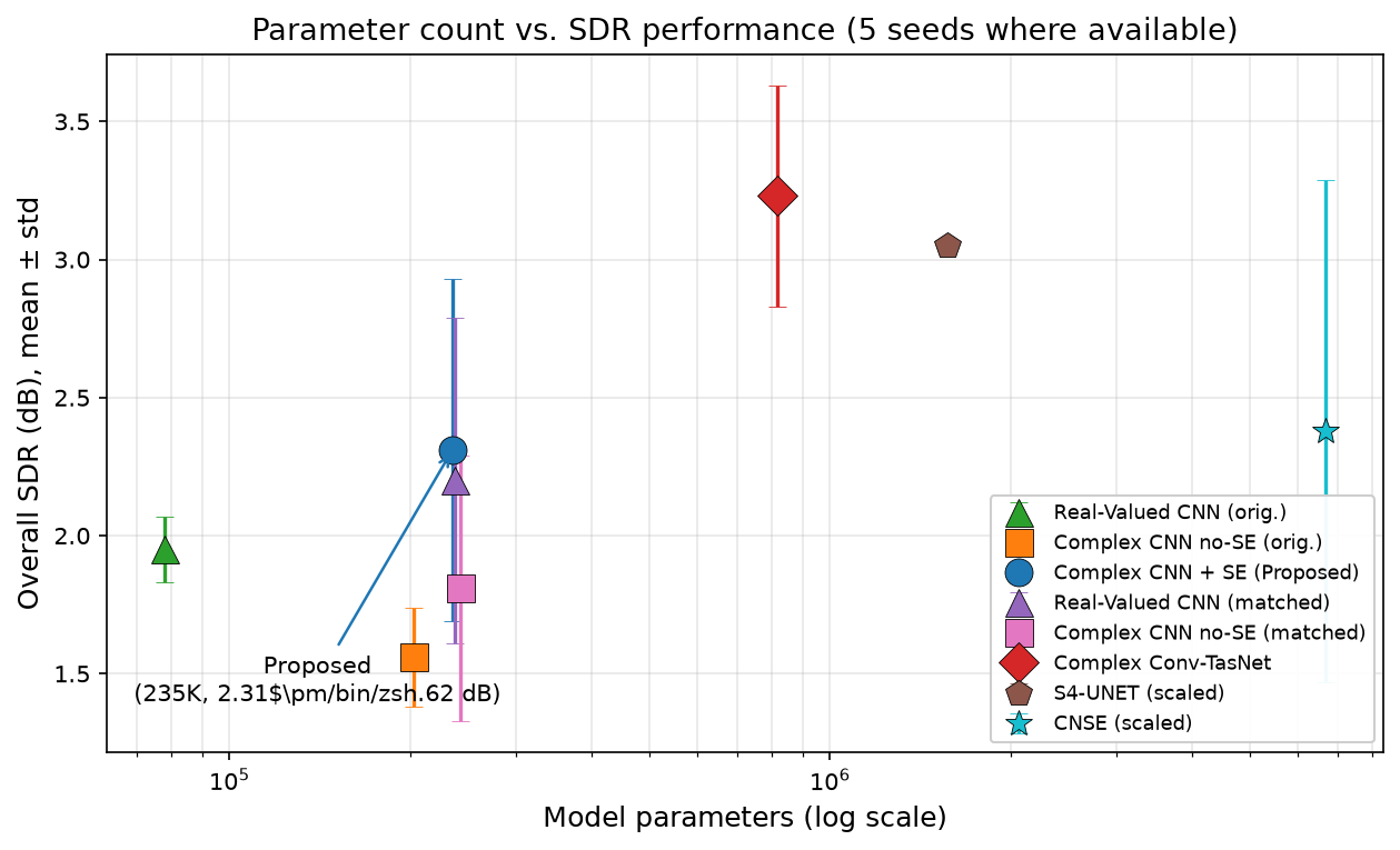
Model	Params	GFLOPs	GPU (ms)	CPU (ms)	Peak mem (MB)	Throughput (bs=1)
Complex CNN + SE (Proposed)	235K	3.27	2.43	30.9	170	438 /s
Complex CNN (no SE)	203K	3.27	1.89	32.8	169	553 /s
Real-Valued CNN	78K	1.26	0.39	5.0	57	2,652 /s
Complex Conv-TasNet	817K	12.76	9.54	40.6	60	105 /s

The proposed C-SE improves single-sample latency ($2.43$ ms vs. $9.54$ ms for Conv-TasNet) and parameter count while trading off activation memory (170 MB vs. 60 MB) and batched throughput. The real-valued baseline at 78K params has the highest throughput by a wide margin; the SE block's 32-channel sigmoid FC adds non-trivial cost at $bs \ge 16$.

08

Discussion & Limitations

A frank accounting of what this paper does and does not claim.

Is the +0.50 dB C-SE gain real, or could it be seed luck?

Honest answer: the paired Wilcoxon $p$-value is $0.125$, which does not reach $\alpha = 0.05$. With only 5 paired seeds the smallest attainable two-sided $p$ is $0.0625$ (achieved against the matched real-valued baseline). We do not claim C-SE is statistically superior; we claim it is a competitive operating point on the dimensions of partial collapse-resistance, per-parameter efficiency, and predictable runtime.

Why is the cross-domain comparison not "fair"?

CNSE and S4-UNET were originally designed for RTX 5090D (32 GB) and we re-implemented them at scaled-down widths to fit our 8 GB GPU (CNSE 6.69M, S4-UNET 1.57M parameters, vs. the original ~50M for CNSE). The reported numbers should be read as approximate upper-bound comparisons rather than direct reproductions. A per-component fidelity check (HiPPO initialisation, DPLR parameterisation for S4; RP preprocessing for CNSE) is left to future work.

What about real-captured I/Q data?

The synthesis pipeline covers the dominant physical effects (RRC pulse shape + multipath + AWGN + random carrier offsets) but cannot capture hardware imperfections (DC offset, I/Q imbalance, phase noise, AGC dynamics). We ship data_radioml.py as an optional loader for the public RadioML 2016.10A corpus so the community can extend the evaluation. The headline numbers do not use it.

Why only 5 seeds?

Compute budget: 5 seeds for the proposed C-SE and matched baselines is ~32 GPU-hours on the RTX 4060. Conv-TasNet, CNSE, and S4-UNET are limited to 3 seeds each due to the larger model size and longer convergence. The smallest two-sided $p$ at $N=3$ is $0.25$, so the cross-domain comparisons are inherently inconclusive regardless of which seed numbers we picked.

Why is the "complex-valued" choice not stronger?

At the $235 K$-parameter scale the matched real-valued baseline reaches $\text{SDR} = 2.20 \pm 0.59 dB$—only $0.11 dB$ below the proposed C-SE ($p=0.0625$, borderline). The C-SE's main strength is therefore not raw SDR but the combination of (i) lightweight capacity, (ii) complex-domain phase preservation, and (iii) partial collapse-resistance at $235 K$ parameters.

What about higher-order modulations, more than 2 sources, real timing offsets?

All three are left to future work. The architecture should generalise—complex-valued processing is modulation-agnostic—but the model would likely need a wider bottleneck, longer training, or a different mask-head design to handle denser constellations. Real timing offsets require a different data generator and a Symbol-Error-Rate pipeline that can compensate per-sample residual timing drift, which our current SER pipeline cannot.

Limitations, in one paragraph

Only 5 training seeds (3 for cross-domain baselines; a 6th–10th would tighten the paired Wilcoxon estimates). BPSK/QPSK/8PSK/16QAM only (no 64QAM, no OFDM). No real-captured co-frequency data; RadioML 2016.10A shipped as an optional loader. Cross-domain baselines are re-implementations at scaled-down widths, not direct reproductions. Symbol timing is generator-aligned (not real). Output collapse is documented empirically but not theoretically analysed. No claim of statistical dominance over any baseline.

Future directions (from the paper's closing section)

Steering the collapse regime through loss shaping. Add a regulariser that penalises the all-zero-mask solution directly, so the operating point is selected at training time, not at random.
Validation on RadioML 2016.10A and over-the-air captures. The data_radioml.py loader is shipped but not used in headline results; extending the evaluation to a public I/Q corpus is the most important direction.
Open-set modulation mixtures. Train with a mixture of constellations plus a learned modulation-classifier branch to handle real-world traffic where the receiver does not know the source modulations in advance.
Phase-preserving complex attention with polar parameterisation. The complex_mean scale-mode ablation does not constitute a fair test of complex phase. A polar parameterisation that preserves phase by construction is the natural follow-up.
Longer training schedules and more seeds. A 6th–10th seed would tighten the cross-seed standard deviation from 0.62 dB to roughly 0.4 dB; combined with more compute, this would enable Wilcoxon tests with lower attainable $p$-values.

09

Citation

If you use this work, please cite the paper.

BibTeX

@article{nong2026cse,
  title   = {A Lightweight Complex-Valued CNN with Complex
             Squeeze-and-Excitation Attention for Single-Channel
             Blind Source Separation of Co-Frequency Communication
             Signals},
  author  = {Nong, Bin and Fu, Weihong and Jiang, Zhuoyun},
  journal = {Wireless Personal Communications},
  year    = {2026},
  note    = {Under review (R1 $\to$ R2)}
}

Resources

Paper PDF (13 pages, Springer svjour3)
Code paper1_cnn_se/ · PyTorch, single-file training
Interactive viz paper1_viz.html · dark-theme developer walkthrough
Experiment log EXPERIMENT_LOG.md · per-seed numbers for 44 runs across 7 phases
RadioML loader data_radioml.py shipped in paper1_cnn_se/
Hardware Single NVIDIA RTX 4060 (8 GB); ~53 GPU-hours total.
Contact nongbin@tfswufe.edu.cn